
Composition
There are three types of composite available for use in MCAS-S:
- Manual (default):
Allows you to combine data layers using simple weightings. This is the simplest option to combine layers applying a single function to all layers such as adding, multiplying or finding the minimum or maximum (of the classified or raw data). - Function:
If you require more flexibility to combine input layers into a composite map you can enter your own algebraic expression using the function editor. The function editor allows you to treat different input layers in different ways. - Analytical Hierachy Process (AHP):
The AHP option provides a more structured alternative to the simple additive weighting procedure used for Manual composite development. You can use AHP to assess input layers against each other on a pair-wise basis, making judgements of relative importance.
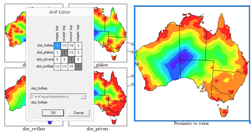
An AHP composite will be used to find Proximity to water.
- Click and Drag the "Composite" tool tip onto the workspace. This will generate an empty composite layer.
- Select the composite and rename it to "Proximity to water" in the "Layer name" field.
- In the "Weighting" section, click the "AHP" radio button.
- Select "dist_fwflats", "dist_plakes", "dist_swflats", and "dist_privers" from the list of input layers. A default AHP composite will be generated.
- Select 10 classes from the "Classes" drop down menu. The classes are already in the correct order so we will not need to allocate the classes in reverse order.
- Click "Edit" (found next to the AHP radio button) and the "AHP Editor" dialogue box will appear.
- Use the AHP editor matrix to edit pair-wise layer weightings by clicking on the light-grey number boxes in the Editor window, and then by selecting a ranking option from the drop-down menu. You cannot edit dark-grey boxes as these show a layer compared to itself. Example weights can be seen below:
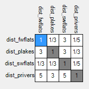
Note that the order in which the attributes appear on the axes in this example may differ from your own, if you are following along, double check your weights. - After entering and checking the layer weightings click OK to display to composite layer in the workspace.
Two-way comparison
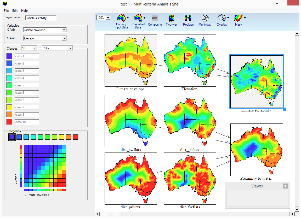
A two-way comparison can be used to explore the spatial association between two data layers. A colour ramp/value scale can be defined to highlight the association of different values of the contributing layers. The two-way comparison is visualised in a dynamic two-dimensional colour matrix.
A two-way will be used to compare the climate envelope of the species and elevation data.
- Click and drag a two-way onto the workspace.
- Rename it to "Climate suitability".
- On the X-Axis, select "Climate envelope".
- On the Y-Axis, select "Elevation".
- Select 10 classes from the "Classes" drop down menu.
- Right-Click a square on the matrix grid (under the "categories" section) to quickly select a focal point.
- You may also select a colour by clicking on the horizontal array of colours above the matrix and manually painting in the squares of the matrix by left clicking them.
As we know that the species much prefers lower elevations and the climate envelope shows the location of ideal climatic conditions, we can weigh the matrix accordingly (see matrix in figure below).
← Previous Section: Input and Classification | Next Section: Building Criteria →